کتاب علوم اعصاب برای هوش مصنوعی؛ حواس به عنوان ورودی پایه

Abstract

From marine animals, insects to humans, we are all limited by the resolution of our senses and rewarded through our senses. Each sense detects and locally processes signals. This Chapter illustrates the neuronal setup of basic senses, all of which can be used as cues for navigation (more in Chapter 7) and associative learning. A variety of animals including insects are already inspiring new algorithms and robotics design. Layers of neurons in the visual cortex inspired AI algorithms, but we now know that they work rather differently. It is probably a universal theme that individual functions are achieved with a relatively small number of neurons.

چکیده

از حیوانات دریایی و حشرات گرفته تا انسان‌ها، همه ما محدود به قدرت تفکیک حواس خود هستیم و از طریق حواس خود پاداش می‌گیریم. هر حس سیگنال‌ها را تشخیص داده و به صورت محلی پردازش می‌کند. این فصل، ساختار عصبی حواس پایه را نشان می‌دهد که همه آنها می‌توانند به عنوان نشانه‌هایی برای ناوبری (بیشتر در فصل 7) و یادگیری تداعی‌گر استفاده شوند. انواع حیوانات از جمله حشرات در حال حاضر الهام‌بخش الگوریتم‌ها و طراحی رباتیک جدید هستند. لایه‌های نورونی در قشر بینایی الهام‌بخش الگوریتم‌های هوش مصنوعی بوده‌اند، اما اکنون می‌دانیم که آنها نسبتاً متفاوت عمل می‌کنند. احتمالاً این یک موضوع جهانی است که عملکردهای فردی با تعداد نسبتاً کمی نورون به دست می‌آیند.

Keywords

Senses, olfaction, sparse network, continual learning, gradient learning, ribbon synapses, vision, data preprocessing, autoencoder, mechanosensory.

کلمات کلیدی

حواس، بویایی، شبکه پراکنده، یادگیری مداوم، یادگیری گرادیانی، سیناپس‌های نواری، بینایی، پیش‌پردازش داده‌ها، رمزگذار خودکار، حسگر مکانیکی.

2.1 Olfaction

۲.۱ حس بویایی

2.1.1     Prioritizing with Separation and Tagging?

Olfaction is an ancient sense that plays key roles in both inverte- brates (e.g., worms, insects) and vertebrates (those that have a spine, from fish to humans). In cockroach, olfactory signals, including pheromones, are locally separated and processed in the antenna, before getting into the brain (Fig. 2.1).

۲.۱.۱     اولویت‌بندی با جداسازی و برچسب‌گذاری؟

بویایی یک حس باستانی است که نقش‌های کلیدی را هم در بی‌مهرگان (مانند کرم‌ها، حشرات) و هم در مهره‌داران (آن‌هایی که ستون فقرات دارند، از ماهی‌ها گرفته تا انسان) ایفا می‌کند. در سوسک، سیگنال‌های بویایی، از جمله فرومون‌ها، قبل از رسیدن به مغز، به صورت محلی جدا شده و در شاخک پردازش می‌شوند (شکل ۲.۱).

Figure 2.1 Separation of olfactory signals in an insect. (A) Schematic illustration of the olfaction pathways from the periphery to higher brain centers in the cockroach protocerebrum. Olfactory sensory neurons (OSNs) of perforated basiconic sensilla (green) run through antennal tracts T1-T4 and terminate in the n-anteroventral group of glomeruli. Projection neurons (PNs) with dendrites in these glomeruli project through the mALT to the protocerebrum. OSNS in trichoid and grooved basiconic sensilla (yellow) run through antennal tracts T5 and T6-10, respectively, and terminate in the n-posterodorsal group of glomeruli. PNs with dendrites in these glomeruli project through the mIALT II to the protocerebrum. L, lateral; mALT, medial antennal lobe tract; MG, macroglomerulus; mlALT II, mediolateral antennal lobe tract; NA, n-anterior; T1-10, antennal tracts 1-10. (B) The number of neurons in each group. Abbreviations as in (A).
Credit: Part A, Fig. 1, and Part B, Fig. 3 of ref. 1.

شکل 2.1 تفکیک سیگنال‌های بویایی در یک حشره. (الف) تصویر شماتیک از مسیرهای بویایی از محیط به مراکز بالاتر مغز در مغز اولیه سوسک. نورون‌های حسی بویایی (OSNs) حسگرهای بازیونیک سوراخ‌دار (سبز) از طریق مسیرهای شاخکی T1-T4 عبور می‌کنند و در گروه n-پیش‌شکمی گلومرول‌ها خاتمه می‌یابند. نورون‌های پروجکشن (PNs) با دندریت‌ها در این گلومرول‌ها از طریق mALT به مغز اولیه امتداد می‌یابند. OSNS در حسگرهای بازیونیک تریکوئید و شیاردار (زرد) به ترتیب از طریق مسیرهای شاخکی T5 و T6-10 عبور می‌کنند و در گروه n-خلفی-پشتی گلومرول‌ها خاتمه می‌یابند. PNs با دندریت‌ها در این گلومرول‌ها از طریق mIALT II به مغز اولیه امتداد می‌یابند. L، جانبی؛ mALT، مسیر لوب شاخکی میانی؛ MG، ماکروگلومرول؛ mlALT II، مسیر لوب شاخکی داخلی-جانبی؛ NA، n-قدامی؛ T1-10، مسیرهای شاخکی 1-10. (ب) تعداد نورون‌ها در هر گروه. اختصارات مانند (الف).
منبع: بخش الف، شکل 1، و بخش ب، شکل 3 از مرجع 1.

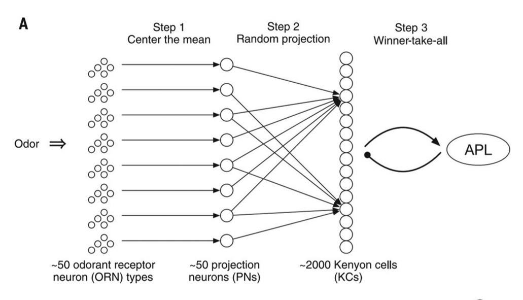
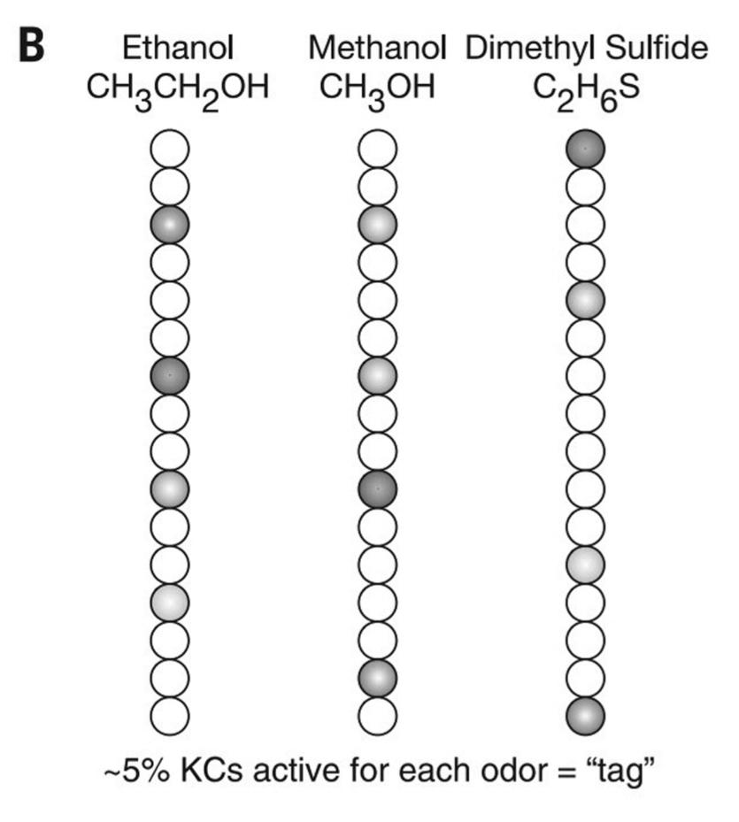
Figure 2.2 Mapping between the fly olfactory circuit and locality-sensitive hashing (LSH). (A) Schematic of the fly olfactory circuit. In step 1, 50 odorant receptor neurons (ORNS) in the fly’s nose send axons to 50 projection neurons (PNs) in the glomeruli; as a result of this projection, each odor is represented by an exponential distribution of firing rates, with the same mean for all odors and all odor concentrations. In step 2, the PNs expand the dimensionality, projecting to 2000 Kenyon cells (KCS) connected by a sparse, binary random projection matrix. In step 3, the KCs receive feedback inhibition from the anterior paired lateral (APL) neuron, which leaves only the top 5% of KCs to remain firing spikes for the odor. This 5% corresponds to the tag (hash) for the odor. (B) Illustrative odor responses. Similar pairs of odors (e.g., methanol and ethanol) are assigned more similar tags than are dissimilar odors. Darker shading denotes higher activity. (C) Differences between conventional LSH and the fly algorithm. In the example, the computational complexity for LSH and the fly are the same. The input dimensionality d = 5. LSH computes m = 3 random projections, each of which requires 10 operations (five multiplications plus five additions). The fly computes m = 15 random projections, each of which requires two addition operations. Thus, both require 30 total operations. x, input feature vector; r, Gaussian random variable; w, bin width constant for discretization.
Credit: Fig. 1 of ref. 4.

شکل 2.2 نقشه‌برداری بین مدار بویایی مگس و هشینگ حساس به محل (LSH). (الف) شماتیک مدار بویایی مگس. در مرحله 1، 50 نورون گیرنده بو (ORNS) در بینی مگس، آکسون‌ها را به 50 نورون افکنش (PN) در گلومرول‌ها می‌فرستند. در نتیجه این تصویرسازی، هر بو با توزیع نمایی از نرخ شلیک، با میانگین یکسان برای همه بوها و همه غلظت‌های بو، نمایش داده می‌شود. در مرحله 2، PNها ابعاد را گسترش می‌دهند و به 2000 سلول کنیون (KCS) که توسط یک ماتریس تصویرسازی تصادفی دوتایی و پراکنده متصل شده‌اند، تصویرسازی می‌کنند. در مرحله 3، KCها مهار بازخوردی از نورون جفت‌شده جانبی قدامی (APL) دریافت می‌کنند، که تنها 5٪ بالایی KCها را برای شلیک سنبله‌ها برای بو باقی می‌گذارد. این 5٪ مربوط به برچسب (هش) برای بو است. (ب) پاسخ‌های بویایی توضیحی. به جفت‌های مشابه بو (مثلاً متانول و اتانول) برچسب‌های مشابه‌تری نسبت به بوهای غیرمشابه اختصاص داده می‌شود. سایه تیره‌تر نشان‌دهنده فعالیت بالاتر است. (ج) تفاوت‌های بین LSH معمولی و الگوریتم مگس. در مثال، پیچیدگی محاسباتی برای LSH و مگس یکسان است. ابعاد ورودی d = 5 است. LSH تعداد m = 3 تصویر تصادفی را محاسبه می‌کند که هر کدام به 10 عملیات (پنج ضرب به علاوه پنج جمع) نیاز دارند. مگس تعداد m = 15 تصویر تصادفی را محاسبه می‌کند که هر کدام به دو عملیات جمع نیاز دارند. بنابراین، هر دو به 30 عملیات کلی نیاز دارند. x، بردار ویژگی ورودی؛ r، متغیر تصادفی گاوسی؛ w، ثابت پهنای دسته برای گسسته‌سازی.
منبع: شکل 1 از مرجع 4.

In general, learning one thing at a time is a prevalent mode in animals, unlike the widely used machine-learning algorithms that try to classify between two or more groups. About 5% of the ~2000 Kenyon cells in a fruit fly are activated by each odor (Fig. 2.2). Architecture of the fruit fly olfactory network (Fig. 2.2) enables lifelong continual learning, with much less catastrophic forgetting than existing continual learning methods using deep neuronal networks such as gradient episodic memory (GEM), elastic weight consolidation (EWC), and brain-inspired replay (BI-R)². The fly olfactory network has been shown to work for natural language processing, with faster training and less memory compared to mainstream algorithms such as global vectors for word representation (Glove)³.

به طور کلی، یادگیری یک چیز در یک زمان، برخلاف الگوریتم‌های یادگیری ماشینی که به طور گسترده استفاده می‌شوند و سعی در طبقه‌بندی بین دو یا چند گروه دارند، یک حالت رایج در حیوانات است. حدود 5٪ از حدود 2000 سلول کنیون در یک مگس میوه توسط هر بو فعال می‌شوند (شکل 2.2). معماری شبکه بویایی مگس میوه (شکل 2.2) یادگیری مداوم مادام العمر را امکان‌پذیر می‌کند، با فراموشی فاجعه‌بار بسیار کمتر از روش‌های یادگیری مداوم موجود که از شبکه‌های عصبی عمیق مانند حافظه اپیزودیک گرادیان (GEM)، تثبیت وزن الاستیک (EWC) و بازپخش الهام گرفته از مغز ²(BI-R) استفاده می‌کنند. نشان داده شده است که شبکه بویایی مگس برای پردازش زبان طبیعی، با آموزش سریع‌تر و حافظه کمتر در مقایسه با الگوریتم‌های اصلی مانند بردارهای جهانی برای نمایش کلمات (Glove)³، کار می‌کند.

2.1.2   The Spatiotemporal Resolution of Olfaction

۲.۱.۲  وضوح مکانی-زمانی بویایی

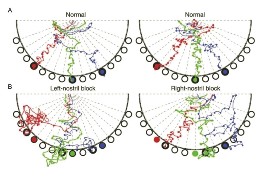
Figure 2.3 Search behavior of moles under normal and nostril-block conditions for radial search paradigm. (A) Normal search behavior from two blind eastern American moles (Scalopus aquaticus, animal no. 2 on left and animal no. 1 on right). Color of the trace matches target well color for each trial. Circles indicate sniffs. The first well explored with a nose dip is indicated by bold outline. (B) Examples of search behavior for left and right-nostril block for cases shown in (A). Left nostril-block biased search to the right, whereas right-nostril block biased search to the left. Colored well indicates target (food) location; bold outline indicates the first well explored. Trace is illustrated until a well was explored, but moles continued to search and found the food in nearly every trial.
Credit: Fig. 2a,b of ref. 10.

شکل ۲.۳ رفتار جستجوی موش‌های کور در شرایط عادی و انسداد سوراخ بینی برای الگوی جستجوی شعاعی. (الف) رفتار جستجوی عادی از دو موش کور کور آمریکایی شرقی (Scalopus aquaticus، حیوان شماره ۲ در سمت چپ و حیوان شماره ۱ در سمت راست). رنگ رد با رنگ چاه هدف برای هر آزمایش مطابقت دارد. دایره‌ها نشان دهنده بو کشیدن هستند. اولین چاهی که با شیب بینی کاوش شده است با طرح پررنگ نشان داده شده است. (ب) نمونه‌هایی از رفتار جستجو برای بلوک سوراخ بینی چپ و راست برای مواردی که در (الف) نشان داده شده است. جستجوی متمایل به سمت راست با بلوک سوراخ بینی چپ، در حالی که جستجوی متمایل به سمت چپ با بلوک سوراخ بینی راست. چاه رنگی نشان دهنده مکان هدف (غذا) است؛ طرح پررنگ نشان دهنده اولین چاه کاوش شده است. رد تا زمانی که یک چاه کاوش شد، نشان داده شده است، اما موش‌های کور به جستجو ادامه دادند و تقریباً در هر آزمایش غذا را پیدا کردند.
منبع: شکل ۲a،b از مرجع ۱۰.

Concentration gradients of odors are key information for spatial navigation of animals including humans ^5-7 (Chapter 7). Odor concentrations (from air that is ~3.5 cm apart for humans) are compared between nostrils⁷. With one nostril blocked, blind moles would eventually locate the odor source after more sidesteps, and often more towards the unblocked side (Fig. 2.3). Each turn after sniffing is like one step in gradient learning (in AI), with smaller steps closer to the odor source (Fig. 2.3).

گرادیان‌های غلظت بوها اطلاعات کلیدی برای جهت‌یابی فضایی حیوانات از جمله انسان‌ها^5-7 هستند  (فصل 7). غلظت بو (از هوایی که برای انسان حدود 3.5 سانتی‌متر فاصله دارد) بین سوراخ‌های بینی⁷ مقایسه می‌شود. با مسدود شدن یک سوراخ بینی، موش‌های کور کور در نهایت پس از گام‌های جانبی بیشتر، و اغلب بیشتر به سمت سمت باز، منبع بو را پیدا می‌کنند (شکل 2.3). هر چرخش پس از بو کشیدن مانند یک گام در یادگیری گرادیان (در هوش مصنوعی) است، با گام‌های کوچکتر نزدیک‌تر به منبع بو (شکل 2.3).

Serial sniffing (e.g., 10 times per second, 10 Hz) is not nearly as fast as the natural temporal variations in odor concentration which can reach 1000 Hz with complex aerodynamics, but mice were shown to be able to distinguish between odor frequencies of up to 40 Hz⁸ (Fig. 2.4). One possibility is that phasing information relative to a wave (Section 7.8) is utilized for distinguishing between such high frequencies.

بو کشیدن سریالی (مثلاً 10 بار در ثانیه، 10 هرتز) به سرعت تغییرات زمانی طبیعی در غلظت بو که می‌تواند با آیرودینامیک پیچیده به 1000 هرتز برسد، نیست، اما نشان داده شده است که موش‌ها می‌توانند فرکانس‌های بو تا 40 هرتز⁸ را تشخیص دهند (شکل 2.4). یک احتمال این است که از اطلاعات فازبندی نسبت به یک موج (بخش 7.8) برای تمایز بین چنین فرکانس‌های بالایی استفاده شود.

We mentioned in Chapter 1 that the forebrain functions primarily in olfaction in fish (Figs. 1.1 and 1.2). The olfactory circuits can detect correlations and anticorrelations (a first step towards causality⁹, Chapter 9), and can separate the sources of the odors⁸.

در فصل ۱ اشاره کردیم که مغز پیشین در ماهی‌ها عمدتاً در حس بویایی نقش دارد (شکل‌های ۱.۱ و ۱.۲). مدارهای بویایی می‌توانند همبستگی‌ها و ضد همبستگی‌ها را تشخیص دهند (اولین قدم به سوی علیت^۹، فصل ۹) و می‌توانند منابع بوها را از هم جدا کنند^۸.

2.2 Taste

Taste receptors expressed on the tongue, soft palate and in other places of the body¹¹, contribute to the reward (or aversion) size perceived by an animal in learning (Chapter 9). Detected at millimolar concentrations, sweets mean calories, and they don’t taste as sweet in ice creams. Cats and some bats do not taste sweetness¹². Bitterness is detected by the same family of receptors that detect sweetness, with some receptors specialized for single poisonous compounds and others more generally activated^11,13 Due to genetic variations, phenylthiocarbamide found in vegetables such as brussels sprouts and broccoli tastes bitterer in some people than others^{11, 14}. The low pH detected by the sour taste indicates potential toxicity, i.e., spoiled food. Salts can be either nutritious or harmful, depending on the concentration¹². Some fat that is useful for female fruit flies can be sweet at low concentrations but bitter at high concentrations¹⁵. In the same type of taste bud cells as sweet and bitter, the Umami taste in humans detects 5′-ribonucleotides, glutamate and aspartate (the mice receptor responds to most L-amino acids¹²) which are both a nitrogen source and a carbon source. The Chinese character for Umami is fish and goat. Ancestors of the Giant Panda lost the Umami receptor as they specialized in bamboo^{16, 17}, so it would be maintaining its nitrogen balance in some other way. Pungency is detected by heat-activated cation channels related to pain sensation¹¹. Astringency, a dry, rough or puckering mouthfeel, is likely due to tactile sensation of aggregation of lubricant proteins in the saliva (due to chemicals in wine, tea, unripe fruit, etc.)¹⁸.

۲.۲ چشایی

گیرنده‌های چشایی که روی زبان، کام نرم و سایر نقاط بدن بیان می‌شوند^۱۱، در اندازه پاداش (یا بیزاری) درک شده توسط یک حیوان در یادگیری نقش دارند (فصل ۹). شیرینی‌ها که در غلظت‌های میلی‌مولار تشخیص داده می‌شوند، به معنای کالری هستند و در بستنی‌ها به شیرینی طعم شیرین ندارند. گربه‌ها و برخی از خفاش‌ها طعم شیرینی را نمی‌چشند^۱۲. تلخی توسط همان خانواده گیرنده‌هایی که شیرینی را تشخیص می‌دهند، تشخیص داده می‌شود، به طوری که برخی از گیرنده‌ها برای ترکیبات سمی منفرد تخصص یافته‌اند و برخی دیگر به طور کلی فعال شده‌اند^۱۱،۱۳ به دلیل تغییرات ژنتیکی، فنیل تیوکاربامید موجود در سبزیجاتی مانند کلم بروکسل و کلم بروکلی در برخی افراد تلخ‌تر از دیگران است^۱۱،۱۴. pH پایین تشخیص داده شده توسط طعم ترش، نشان دهنده سمیت بالقوه، یعنی غذای فاسد است. نمک‌ها بسته به غلظت می‌توانند مغذی یا مضر باشند^۱۲. برخی از چربی‌هایی که برای مگس‌های میوه ماده مفید هستند، می‌توانند در غلظت‌های پایین شیرین باشند اما در غلظت‌های بالا تلخ باشند^۱۵. در همان نوع سلول‌های جوانه چشایی که شیرینی و تلخی را تشخیص می‌دهند، طعم اومامی در انسان، 5′-ریبونوکلئوتید، گلوتامات و آسپارتات را تشخیص می‌دهد (گیرنده موش به اکثر اسیدهای آمینه L پاسخ می‌دهد¹²) که هم منبع نیتروژن و هم منبع کربن هستند. کلمه چینی اومامی، ماهی و بز است. اجداد پاندای غول‌پیکر گیرنده اومامی را از دست دادند زیرا در بامبو تخصص یافتند^{16، 17}، بنابراین تعادل نیتروژن خود را به روش دیگری حفظ می‌کردند. تندی توسط کانال‌های کاتیونی فعال شده با گرما مرتبط با حس درد تشخیص داده می‌شود¹¹. گس بودن، احساس خشکی، زبری یا جمع شدن در دهان، احتمالاً به دلیل حس لامسه تجمع پروتئین‌های روان‌کننده در بزاق (به دلیل مواد شیمیایی موجود در شراب، چای، میوه نارس و غیره)¹⁸ است.

Figure 2.4 Distinguishing fast odor stimuli with slow olfactory sensory neurons (OSNs). (A) Membrane voltage relative to baseline of a single model OSN in response to a 10 ms odor pulse. Black traces are individual trials; red trace is average over 20 trials. OSN spike threshold has been set high enough to prevent spiking to illustrate the subthreshold voltage time course. (B) Membrane voltages (gray traces) of ten OSNs from a population of 5,000 in response to a paired odor pulse with pulse width 10 ms and paired pulse interval (PPI) of 25 ms. The voltage time course for one example OSN is in black. Several OSNS reach the OSN spike threshold (dashed red line) and are temporarily reset to the refractory voltage of -1. The population average membrane voltage (red) reveals membrane charging in response to odor stimulation and the subsequent discharging and refractory period. (C) Raster showing the spike times (dots) of the full population from band the corresponding mean firing rate (trace) estimated in 1 ms bins. (D) Mean firing rates computed over 20 trials in response to paired odor pulses of width 10 ms and PPIs of 10 ms (green) and 25 ms (black). (E) Model calcium signals are produced by squaring the instantaneous mean firing rate and filtering the result with a calcium imaging kernel. (F) Model calcium responses to the paired odor stimulus with a PPI of 10 ms (green) and 25 ms (black). Thin traces are single trials, thick traces are averages over 15 trials. (G) Schematic of the OSN model. Variables in dashed bounding boxes are changed for each glomerulus⁸. (H) Linear classifier analysis over an increasing subset size of glomeruli (1-100; plotted is mean ± s.d., 256 repeats for random subsets of n glomeruli generating 256 unshuffled and 256 shuffled accuracies).
Credit: Extended Fig. 1 of ref. 8.

شکل 2.4 تمایز محرک‌های بویایی سریع با نورون‌های حسی بویایی (OSN) کند. (الف) ولتاژ غشا نسبت به خط پایه یک OSN مدل واحد در پاسخ به یک پالس بویایی 10 میلی‌ثانیه. ردهای سیاه آزمایش‌های جداگانه هستند؛ رد قرمز میانگین بیش از 20 آزمایش است. آستانه جهش OSN به اندازه کافی بالا تنظیم شده است تا از جهش جلوگیری شود تا سیر زمانی ولتاژ زیرآستانه را نشان دهد. (ب) ولتاژهای غشا (ردهای خاکستری) ده OSN از یک جمعیت 5000 تایی در پاسخ به یک پالس بویایی جفت شده با پهنای پالس 10 میلی‌ثانیه و فاصله پالس جفت شده (PPI) 25 میلی‌ثانیه. سیر زمانی ولتاژ برای یک OSN نمونه به رنگ سیاه است. چندین OSNS به آستانه جهش OSN (خط قرمز خط‌چین) می‌رسند و به طور موقت به ولتاژ مقاوم -1 بازنشانی می‌شوند. ولتاژ غشای متوسط ​​جمعیت (قرمز) شارژ غشا را در پاسخ به تحریک بو و دوره تخلیه و مقاوم بعدی نشان می‌دهد. (ج) رستر که زمان‌های اوج (نقطه) جمعیت کامل را از باند میانگین نرخ شلیک مربوطه (ردیابی) که در بازه‌های ۱ میلی‌ثانیه‌ای تخمین زده شده است، نشان می‌دهد. (د) میانگین نرخ شلیک محاسبه شده طی ۲۰ آزمایش در پاسخ به پالس‌های بویایی جفت شده با عرض ۱۰ میلی‌ثانیه و PPI های ۱۰ میلی‌ثانیه (سبز) و ۲۵ میلی‌ثانیه (سیاه). (ه) سیگنال‌های کلسیم مدل با به توان دو رساندن میانگین نرخ شلیک آنی و فیلتر کردن نتیجه با یک هسته تصویربرداری کلسیم تولید می‌شوند. (و) پاسخ‌های کلسیم مدل به محرک بویایی جفت شده با PPI ۱۰ میلی‌ثانیه (سبز) و ۲۵ میلی‌ثانیه (سیاه). ردهای نازک، آزمایش‌های تکی هستند، ردهای ضخیم، میانگین‌های ۱۵ آزمایش هستند. (ز) شماتیک مدل OSN. متغیرهای داخل کادرهای مرزی خط‌چین برای هر گلومرول⁸ تغییر می‌کنند. (ح) تحلیل طبقه‌بندی خطی روی یک زیرمجموعه رو به افزایش از گلومرول‌ها (۱-۱۰۰؛ نمودار رسم شده میانگین ± انحراف معیار است، ۲۵۶ تکرار برای زیرمجموعه‌های تصادفی از n گلومرول که ۲۵۶ دقت بدون تغییر و ۲۵۶ دقت با تغییر ایجاد می‌کند).
منبع: شکل ۱ بسط‌یافته از مرجع ۸.

2.3 Hearing

Unlike visual scenes in the environment, sounds always mean that someone or something has made the sound¹⁹. If a group of animals are calling, one has to know what to do. We can attest to the distracting nature of unattended auditory information that is also processed. In primates like us, a lot of spectral details are already lost at the cochlea in the inner ear, with a roughly logarithmic representation of increasing frequency of sound¹⁹. Mechanotransduction at the bundled ciliates of hair cells rapidly generates changing receptor potentials, but this changing signal is limited by the membrane time constant. Instead of the classic point-to-point transduction at synapses (Chapter 1), hair cells in the inner ear, as well as rods and cones in the retina, have ribbon synapses that enable persistent activity²⁰ (Fig. 2.5).

۲.۳ شنوایی

برخلاف صحنه‌های بصری در محیط، صداها همیشه به این معنی هستند که کسی یا چیزی صدا را ایجاد کرده است^۱۹. اگر گروهی از حیوانات صدا می‌زنند، باید بدانیم چه باید بکنیم. می‌توانیم ماهیت حواس‌پرتی اطلاعات شنیداریِ بدون توجه که پردازش نیز می‌شوند را تأیید کنیم. در نخستی‌سانانی مانند ما، بسیاری از جزئیات طیفی در حلزون گوش داخلی از بین رفته‌اند، با نمایش تقریباً لگاریتمی از افزایش فرکانس صدا^۱۹. انتقال مکانیکی در مژک‌های دسته‌ای سلول‌های مو به سرعت پتانسیل‌های گیرنده متغیری ایجاد می‌کند، اما این سیگنال متغیر توسط ثابت زمانی غشا محدود می‌شود. به جای انتقال کلاسیک نقطه به نقطه در سیناپس‌ها (فصل ۱)، سلول‌های مو در گوش داخلی و همچنین میله‌ها و مخروط‌ها در شبکیه، سیناپس‌های روبانی دارند که فعالیت مداوم را ممکن می‌سازند^۲۰ (شکل ۲.۵).

Differences in sound intensity, time delay and phase between the two ears can all be useful for locating the direction of the sound21 (Fig. 2.6). The spatial resolution in the horizontal plane is highest around the interaural midline in front of an individual and deteriorates towards the acoustic periphery, especially behind one’s back. The posterior auditory cortex responds faster, while the anterior auditory cortex has a more sustained activity¹⁹, ²¹ (Fig. 2.6).

تفاوت در شدت صدا، تأخیر زمانی و فاز بین دو گوش، همگی می‌توانند برای تعیین جهت صدا ۲۱ مفید باشند (شکل ۲.۶). وضوح فضایی در صفحه افقی در اطراف خط میانی بین دو گوش در جلوی فرد بیشترین مقدار را دارد و به سمت حاشیه صوتی، به ویژه پشت سر، کاهش می‌یابد. قشر شنوایی خلفی سریع‌تر پاسخ می‌دهد، در حالی که قشر شنوایی قدامی فعالیت پایدارتری دارد^{19، 21} (شکل 2.6).

Auditory hallucinations are common for patients with conditions such as schizophrenia and bipolar disorders (Fig. 2.7), whereas Parkinson’s disease patients treated with L-dopa could have visual and auditory hallucinations ²², ²³. Injuries in the auditory cortex did not result in deafness, but the patients became “word deaf” and can no longer process the structure information in sound (more on language in Chapter 8).

توهمات شنیداری در بیماران مبتلا به بیماری‌هایی مانند اسکیزوفرنی و اختلالات دوقطبی رایج است (شکل 2.7)، در حالی که بیماران مبتلا به پارکینسون که با L-dopa درمان می‌شوند، می‌توانند توهمات بینایی و شنوایی داشته باشند ^{22، 23}. آسیب‌های قشر شنوایی منجر به ناشنوایی نشد، اما بیماران “ناشنوا نسبت به کلمات” شدند و دیگر نمی‌توانند اطلاعات ساختاری صدا را پردازش کنند (بیشتر در مورد زبان در فصل 8).

Figure 2.5 Ribbon synapses in the inner ear and the retina. With one or more “ribbon” anchored presynaptically, glutamate can be persistently released in the active zone. Left: Signals from inner hair cells (IHC) go through ribbon synapses with spiral ganglion cells (SGN). Deflection of hair bundles activates mechanosensitive channels on the hair cells of the auditory and vestibular epithelia of the inner ear, which then release multiple doses of glutamate to the SGN. Right: Photon-induced isomerization of retinal hyperpolarize rods and cones, which then signal to bipolar cells through ribbon synapses. Bipolar cells again have ribbon synapses to signal to amacrine and ganglion cells in the inner retina.
Credit: From Abstract of ref. 20.

شکل 2.5 سیناپس‌های روبانی در گوش داخلی و شبکیه. با یک یا چند “روبان” که به صورت پیش‌سیناپسی لنگر انداخته‌اند، گلوتامات می‌تواند به طور مداوم در منطقه فعال آزاد شود. سمت چپ: سیگنال‌های سلول‌های مویی داخلی (IHC) از طریق سیناپس‌های روبانی با سلول‌های گانگلیون مارپیچی (SGN) عبور می‌کنند. انحراف دسته‌های مو، کانال‌های حساس به مکان را روی سلول‌های مویی اپیتلیوم شنوایی و دهلیزی گوش داخلی فعال می‌کند که سپس دوزهای متعددی از گلوتامات را به SGN آزاد می‌کنند. راست: ایزومریزاسیون القایی فوتونی سلول‌های استوانه‌ای و مخروطی فوق قطبی شبکیه، که سپس از طریق سیناپس‌های روبانی به سلول‌های دوقطبی سیگنال می‌دهند. سلول‌های دوقطبی نیز سیناپس‌های روبانی برای سیگنال‌دهی به سلول‌های آماکرین و گانگلیونی در شبکیه داخلی دارند.
منبع: از چکیده مرجع ۲۰.

Figure 2.6 The physiological range of interaural phase differences (IPD) is a function of sound frequency, head size and temporal resolution of the auditory system. For periodic tones, interaural time differences (ITD) up to half the period of the tone can be expressed in terms of phase shifts, i.e., IPD. (A) Detection of IPD depends on head size. Humans have a relatively large head size and IPD is more useful than ILD (interaural level (intensity) difference) only for low frequencies, which include the frequency of speech. The legend for high-frequency and low-frequency pure tones have been swapped from ref. 21. (B) Besides head size, IPD is also limited by the temporal resolution of the auditory system, i.e., the highest frequency to which the firing of auditory nerve fibers and neurons at subsequent stages in the subcortical auditory pathway can phase lock, which reaches 10 kHz in barn owls. Credit: From Box 1 of ref. 21.

شکل 2.6 محدوده فیزیولوژیکی اختلاف فاز بین گوشی (IPD) تابعی از فرکانس صدا، اندازه سر و تفکیک زمانی سیستم شنوایی است. برای صداهای تناوبی، اختلاف زمان بین گوشی (ITD) تا نصف دوره تناوب صدا را می‌توان بر حسب تغییرات فاز، یعنی IPD، بیان کرد. (الف) تشخیص IPD به اندازه سر بستگی دارد. انسان‌ها اندازه سر نسبتاً بزرگی دارند و IPD فقط برای فرکانس‌های پایین، که شامل فرکانس گفتار می‌شود، مفیدتر از ILD (اختلاف سطح (شدت) بین گوشی) است. راهنمای مربوط به صداهای خالص با فرکانس بالا و فرکانس پایین از مرجع 21 جابجا شده است. (ب) علاوه بر اندازه سر، IPD همچنین توسط تفکیک زمانی سیستم شنوایی محدود می‌شود، یعنی بالاترین فرکانسی که شلیک فیبرها و نورون‌های عصبی شنوایی در مراحل بعدی در مسیر شنوایی زیرقشری می‌تواند قفل فاز شود، که در جغدهای انبار به 10 کیلوهرتز می‌رسد. منبع: از کادر 1 مرجع 21.

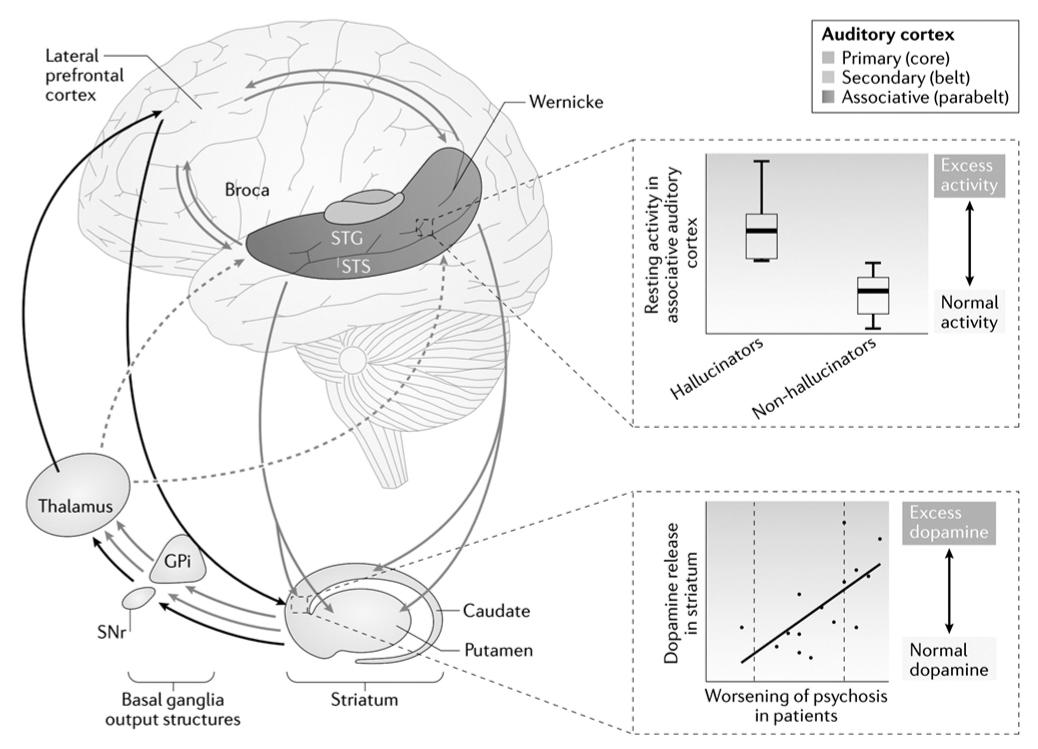
Figure 2.7 Circuitry of associative auditory cortex and basal ganglia relevant to perceptual disturbances in psychosis. The anatomy of auditory cortex and the downstream projections of associative auditory cortex to prefrontal cortex and striatum, as well as the cortico-cortical loops and cortico-basal ganglia-thalamocortical loops proposed to be relevant for perceptual disturbances. In the center, a lateral surface of the brain is shown, indicating the different areas of auditory cortex in different colors. The associative auditory cortex features a gradient from anterior-ventral to posterior-dorsal aspects. Connections from these aspects of the associative auditory cortex to the dorsal striatum and lateral prefrontal cortex are indicated by arrows reflecting the colors of the areas of origin. Note that the striatum, basal ganglia and thalamus output structures are in the center of the brain, but here they are shown separately for illustrative purposes. Prefrontal inputs are also shown as gray arrows. Outputs from the striatum to basal ganglia output structures and the thalamus are also illustrated, in addition to thalamocortical projections back to the areas where the inputs originate. Dashed arrows indicate connections that have not been fully described in primates. Findings of increased activity in associative auditory cortex in relation to hallucinations and increased striatal dopamine in psychosis are depicted as inserts.
Credit: From Fig. 4a of ref. 23.

شکل ۲.۷ مدار قشر شنوایی تداعی‌گر و عقده‌های قاعده‌ای مرتبط با اختلالات ادراکی در روان‌پریشی. آناتومی قشر شنوایی و انشعابات پایین‌دست قشر شنوایی تداعی‌گر به قشر پیش‌پیشانی و جسم مخطط، و همچنین حلقه‌های قشری-قشری و حلقه‌های قشری-قشری-عقده‌های قاعده‌ای-تالاموکورتیکال که پیشنهاد می‌شود با اختلالات ادراکی مرتبط باشند. در مرکز، یک سطح جانبی مغز نشان داده شده است که نواحی مختلف قشر شنوایی را با رنگ‌های مختلف نشان می‌دهد. قشر شنوایی تداعی‌گر دارای یک شیب از جنبه‌های قدامی-شکمی به خلفی-پشتی است. اتصالات از این جنبه‌های قشر شنوایی تداعی‌گر به جسم مخطط پشتی و قشر پیش‌پیشانی جانبی با فلش‌هایی که رنگ نواحی مبدا را منعکس می‌کنند، نشان داده شده‌اند. توجه داشته باشید که جسم مخطط، عقده‌های قاعده‌ای و ساختارهای خروجی تالاموس در مرکز مغز قرار دارند، اما در اینجا آنها به طور جداگانه برای اهداف توضیحی نشان داده شده‌اند. ورودی‌های پیش‌پیشانی نیز به صورت فلش‌های خاکستری نشان داده شده‌اند. خروجی‌های جسم مخطط به ساختارهای خروجی عقده‌های قاعده‌ای و تالاموس نیز نشان داده شده‌اند، علاوه بر این، پیش‌بینی‌های تالاموکورتیکال به مناطقی که ورودی‌ها از آنها سرچشمه می‌گیرند، نشان داده شده‌اند. فلش‌های خط‌چین نشان‌دهنده ارتباطاتی هستند که به طور کامل در نخستی‌سانان توصیف نشده‌اند. یافته‌های افزایش فعالیت در قشر شنوایی مرتبط با توهم و افزایش دوپامین جسم مخطط در روان‌پریشی به صورت درج نشان داده شده‌اند.
منبع: از شکل 4a از مرجع 23.

2.4 Visual Signal Processing in Each Cell

Vision is a dominant sense in many animals. Among the rods and cone photoreceptor cells in the retina (Fig. 2.5), the cones detect colors, and motion blur that can be decoded for movements²⁴.

۲.۴ پردازش سیگنال بصری در هر سلول

بینایی حس غالب در بسیاری از حیوانات است. در میان سلول‌های گیرنده نوری استوانه‌ای و مخروطی در شبکیه (شکل ۲.۵)، مخروط‌ها رنگ‌ها و تاری حرکتی را که می‌توانند برای حرکات رمزگشایی شوند، تشخیص می‌دهند^۲۴.

Figure 2.8 Mice learning two visual categories with neuronal activities in the visual cortex. (A) Mice learn discriminating information-integration categories in a touch screen operant chamber. Touch screens (v) display visual stimuli and record screen presses, two at a time from a total of 42 grating stimuli that differed in orientation and spatial frequency. Food pellet rewards (r) are delivered via a pellet feeder into a dish, after each correct choice of the rewarded category, and not the other category. A drinking bottle, house light, speaker, and lever are positioned on the east and south walls. (B) Mean (ts.e.m.) learning curve. Gray lines represent individual animals (n = 8 mice). Latin numerals denote category training stages. Insets show active stimuli (black) and not-yet-introduced stimuli (gray). (C,D) With head fixed for chronic calcium imaging, unlike in (A), only one visual stimulus was shown each time, and the mouse’s choice was indicated by licking for a water reward. (C) Fraction of stimulus- and task-activated responsive neurons (corrected for variable trial numbers by subsampling). The y axis shows visual areas with chronic recordings, and the x axis shows imaging time points. TC, out-of-task time points (tuning curves). Task, in-task time points. L, separates baseline from after category learning. The second in- task baseline was only acquired in a subset of mice. (D) Map of mouse visual areas (based on ref. 25) showing the fraction of cluster 1 and cluster 2 (k-means clustering) chronic recordings per area after category learning²⁶. V1, primary visual cortex; LM, lateromedial area; LI, laterointermediate area; AL, anterolateral area; RL, rostrolateral area; AM, anteromedial area; PM, posteromedial area; P, posterior; POR, postrhinal. The mouse V1 has direct input to other visual areas, while only V2, V3, V4 and the middle temporal area (MT) are known to receive substantial V1 input in the primate brain²⁵.
Credit: Part A,B from Fig. 1a,b and Part C,D from Fig. 4a,d of ref. 26.

شکل 2.8 موش‌ها در حال یادگیری دو دسته بصری با فعالیت‌های عصبی در قشر بینایی. (الف) موش‌ها دسته‌های ادغام اطلاعات تفکیکی را در یک محفظه عملگر صفحه لمسی یاد می‌گیرند. صفحات لمسی (v) محرک‌های بصری را نمایش می‌دهند و فشار دادن صفحه را ثبت می‌کنند، دو تا در یک زمان از مجموع 42 محرک توری که در جهت‌گیری و فرکانس فضایی متفاوت بودند. پاداش‌های گلوله‌های غذایی (r) از طریق یک تغذیه‌کننده گلوله به یک ظرف، پس از هر انتخاب صحیح از دسته پاداش داده شده، و نه دسته دیگر، تحویل داده می‌شوند. یک بطری نوشیدنی، چراغ خانه، بلندگو و اهرم روی دیوارهای شرقی و جنوبی قرار گرفته‌اند. (ب) میانگین (ts.e.m.) منحنی یادگیری. خطوط خاکستری نشان دهنده حیوانات منفرد (n = 8 موش) هستند. اعداد لاتین مراحل آموزش دسته را نشان می‌دهند. خطوط داخلی محرک‌های فعال (سیاه) و محرک‌های هنوز معرفی نشده (خاکستری) را نشان می‌دهند. (C، D) با ثابت بودن سر برای تصویربرداری کلسیم مزمن، برخلاف (A)، هر بار فقط یک محرک بصری نشان داده می‌شد و انتخاب موش با لیسیدن برای پاداش آب نشان داده می‌شد. (ج) کسری از نورون‌های پاسخگو فعال‌شده توسط محرک و وظیفه (با نمونه‌گیری فرعی برای تعداد آزمایش‌های متغیر اصلاح شده است). محور y نواحی بینایی با ثبت‌های مزمن را نشان می‌دهد و محور x نقاط زمانی تصویربرداری را نشان می‌دهد. TC، نقاط زمانی خارج از وظیفه (منحنی‌های تنظیم). وظیفه، نقاط زمانی در حین وظیفه. L، خط پایه را از بعد از یادگیری دسته‌بندی جدا می‌کند. خط پایه دوم در حین وظیفه فقط در زیرمجموعه‌ای از موش‌ها به دست آمد. (د) نقشه نواحی بینایی موش (بر اساس مرجع 25) که کسری از ثبت‌های مزمن خوشه‌ای 1 و خوشه‌ای 2 (خوشه‌بندی k-means) را در هر ناحیه پس از یادگیری دسته‌بندی نشان می‌دهد26. V1، قشر بینایی اولیه؛ LM، ناحیه جانبی-میانی؛ LI، ناحیه جانبی-میانی؛ AL، ناحیه قدامی-جانبی؛ RL، ناحیه روسترو-جانبی؛ AM، ناحیه قدامی-میانی؛ PM، ناحیه خلفی-میانی؛ P، خلفی؛ POR، خلفی-بینی. ناحیه V1 موش ورودی مستقیم به سایر نواحی بینایی دارد، در حالی که مشخص شده است که فقط V2، V3، V4 و ناحیه گیجگاهی میانی (MT) ورودی قابل توجهی از V1 را در مغز نخستی‌ها دریافت می‌کنند²⁵.
منبع: قسمت A، B از شکل 1a، b و قسمت C، D از شکل 4a، d از مرجع 26.

Figure 2.9 Responses of single neurons are well explained by single disentangled latent units. (A) Coronal section showing the location of fMRI- identified face patches in two primates, with patch AM (anteromedial area) circled in red. Dark black lines, electrodes. (B) Explained variance of single neuron responses to 2,100 faces. Response variance in single neurons is explained primarily by single disentangled units encoding different semantically meaningful information, using a deep unsupervised generative model, B-variational autoencoder (beta-VAE). Insets, latent traversals were used to visualize the semantic meaning encoded by single disentangled latent units of a trained model.
Credit: Fig. 2 of ref. 27.

شکل ۲.۹ پاسخ‌های نورون‌های منفرد به خوبی توسط واحدهای نهفته‌ی منفردِ جدا شده توضیح داده می‌شوند. (الف) برش تاجی که محل تکه‌های چهره‌ی شناسایی‌شده توسط fMRI را در دو نخستی نشان می‌دهد، با تکه‌ی AM (ناحیه‌ی قدامی-میانی) که با رنگ قرمز دایره شده است. خطوط سیاه تیره، الکترودها. (ب) واریانس توضیح داده‌شده‌ی پاسخ‌های نورون‌های منفرد به ۲۱۰۰ چهره. واریانس پاسخ در نورون‌های منفرد در درجه‌ی اول توسط واحدهای منفردِ جدا شده که اطلاعات معنادار معنایی متفاوتی را رمزگذاری می‌کنند، با استفاده از یک مدل تولیدی عمیق بدون نظارت، خودرمزگذار B-variational (beta-VAE) توضیح داده می‌شود. از درون‌دادها، پیمایش‌های نهفته برای تجسم معنای معنایی رمزگذاری‌شده توسط واحدهای نهفته‌ی منفردِ جدا شده از یک مدل آموزش‌دیده استفاده شد.
منبع: شکل ۲ از مرجع. ۲۷.

Different areas of the visual cortex (with hundreds to low thousands of neurons in each area in mice) already differ in sensitivity for different features, and there are crosstalk between areas ^{25, 28, 29}. Mice readily learn categories of visual stimuli in the first few trials, using a fraction of the neurons (Fig. 2.8). Intuitively, the category with a food or water reward (or something fearful) might be more important (Fig. 2.8).

نواحی مختلف قشر بینایی (با صدها تا هزاران نورون در هر ناحیه در موش‌ها) از قبل حساسیت متفاوتی برای ویژگی‌های مختلف دارند و بین نواحی ^{۲۵، ۲۸، ۲۹} تداخل وجود دارد. موش‌ها به راحتی دسته‌های محرک‌های بصری را در چند آزمایش اول، با استفاده از کسری از نورون‌ها یاد می‌گیرند (شکل ۲.۸). به طور شهودی، دسته‌ای که پاداش آن غذا یا آب (یا چیزی ترسناک) است، ممکن است مهم‌تر باشد (شکل ۲.۸).

Layer I (L1) of the neocortex mostly contained dendrites from the deeper layers (L2, L3, L5 and occasionally L4^30-32, Fig. 1.9). L1 and L4 of the primary visual cortex (V1) receives input from, and L5-L6 output to evolutionarily more ancient regions such as the thalamus, which includes information on locomotion^{28, 33} (and the thalamus is important both when awake and while asleep, Chapter 6).

لایه I (L1) نئوکورتکس عمدتاً حاوی دندریت‌هایی از لایه‌های عمیق‌تر (L2، L3، L5 و گاهی اوقات L4^30-32، شکل ۱.۹) بود. L1 و L4 قشر بینایی اولیه (V1) ورودی را از مناطق قدیمی‌تر تکاملی مانند تالاموس دریافت می‌کنند، که شامل اطلاعات مربوط به حرکت است ۲۸، ۳۳ (و تالاموس هم در بیداری و هم در خواب مهم است، فصل ۶).

Spontaneous activities in the visual cortex start before eye-opening. Synchronous firing occurs in adjacent neurons sharing similar orientation or spatial frequency preferences in L2-L4 (including excitatory interneurons, i.e., stellate cells, Fig. 1.9) of the visual cortex in rats after eye-opening, whereas neurons in the deeper layers L5-L6 did not get so synchronous with the stimulus ³⁴ (and L6 output to the claustrum ³⁵, Section 7.8). Consistently, adult mice showed more connections within the same layer in the superficial layers than in the deeper layers^36.

فعالیت‌های خودبه‌خودی در قشر بینایی قبل از باز شدن چشم شروع می‌شوند. شلیک همزمان در نورون‌های مجاور که جهت‌گیری یا ترجیحات فرکانس فضایی مشابهی را در L2-L4 (از جمله اینترنورون‌های تحریکی، یعنی سلول‌های ستاره‌ای، شکل 1.9) قشر بینایی در موش‌ها پس از باز شدن چشم دارند، رخ می‌دهد، در حالی که نورون‌های لایه‌های عمیق‌تر L5-L6 با محرک ³⁴ (و خروجی L6 به کلاستروم ³⁵، بخش 7.8) چندان همزمان نشدند. به طور مداوم، موش‌های بالغ اتصالات بیشتری را در همان لایه در لایه‌های سطحی نسبت به لایه‌های عمیق‌تر نشان دادند³⁶.

Single neurons in the visual cortex already encode distinct features of an image, such as the age, smile, hair thickness of a face (Fig. 2.9). We do tend to see smiling faces in objects (searching and hashing, Section 4.4). The face is part of a two- dimensional (2D) continuum of objects recognized: animate versus inanimate in one dimension, stubby (round) versus spiky in the other dimension (Fig. 2.10, more speculations on written language in Section 8.7). Such an arrangement is likely both genetic and stimulus-modulated³⁷. Puppies got to see human faces no later than they open their eyes and see their mother, and learned to read our facial expressions. Animals that look alike to us can look rather unique to each other. Fish³⁸ and birds have many neighbors. Crayfish have been shown to recognize a fight opponent, according to spots and head width³⁹.

نورون‌های منفرد در قشر بینایی، ویژگی‌های متمایز یک تصویر، مانند سن، لبخند، ضخامت موی صورت را رمزگذاری می‌کنند (شکل ۲.۹). ما تمایل داریم چهره‌های خندان را در اشیاء ببینیم (جستجو و هش کردن، بخش ۴.۴). چهره بخشی از یک پیوستار دوبعدی (۲D) از اشیاء شناخته شده است: جاندار در مقابل بی‌جان در یک بعد، کوتاه (گرد) در مقابل تیز در بعد دیگر (شکل ۲.۱۰، گمانه‌زنی‌های بیشتر در مورد زبان نوشتاری در بخش ۸.۷). چنین ترتیبی احتمالاً هم ژنتیکی و هم تنظیم‌شده توسط محرک است^۳۷. توله سگ‌ها می‌توانند چهره‌های انسان را درست قبل از باز کردن چشمانشان و دیدن مادرشان ببینند و یاد بگیرند که حالات چهره ما را بخوانند. حیواناتی که برای ما شبیه به هم هستند، می‌توانند نسبت به یکدیگر نسبتاً منحصر به فرد به نظر برسند. ماهی‌ها^۳۸ و پرندگان همسایگان زیادی دارند. نشان داده شده است که خرچنگ‌های دریایی، بر اساس خال‌ها و عرض سر، حریف جنگی را تشخیص می‌دهند^۳۹.

Objects can also be reconstructed from signals recorded in single neurons, together with a database of labelled images (Fig. 2.11; our brain is also probably generative according to a database, Section 7.8). Thus, if there are scratches on one’s photo (Fig. 2.12), our brain probably detects the scratches and the face with separate cells, unlike the statistical averaging approaches developed by data scientists.

اشیاء همچنین می‌توانند از سیگنال‌های ثبت‌شده در نورون‌های منفرد، همراه با یک پایگاه داده از تصاویر برچسب‌گذاری‌شده، بازسازی شوند (شکل ۲.۱۱؛ مغز ما نیز احتمالاً طبق یک پایگاه داده، بخش ۷.۸، مولد است). بنابراین، اگر روی عکس کسی خراش‌هایی وجود داشته باشد (شکل ۲.۱۲)، مغز ما احتمالاً خراش‌ها و چهره را با سلول‌های جداگانه تشخیص می‌دهد، برخلاف رویکردهای میانگین‌گیری آماری که توسط دانشمندان داده توسعه داده شده‌اند.

Figure 2.10 The neural code for object identity in general. (A) Schematic showing the four quadrants spanned by the first two principal components (PCs) of object space, animate-inanimate (PC1) and stubby-spiky (PC2). The stimuli in each of the quadrants were used for mapping four networks (face patches, body patches, spiky patches and stubby patches) using functional MRI. (B) Projection of preferred axis of each cell (n = 482) onto PC1 versus PC2 for all neurons recorded across four networks (spiky network: orange, body network: lime, face network: green, stubby network: blue). (C) Schematic showing the threefold-repeated topographic map in the monkey inferotemporal cortex that is organized according to the four quadrants of object space. In humans, the fusiform gyrus (Brodmann Area 37) appeared more rolled into the bottom of the lobe (e.g., ref. 40), reminiscent of the different configuration of the hippocampus (Fig. 1.6).
Credit: Fig. 6a,b,c of ref. 41, (A) and (B) were adapted by ref. 41 from ref. 42.

شکل 2.10 کد عصبی برای هویت شیء به طور کلی. (الف) شماتیکی که چهار ربع را نشان می‌دهد که توسط دو مؤلفه اصلی اول (PC) فضای شیء، جاندار-بی‌جان (PC1) و کنده-خاردار (PC2) پوشانده شده است. محرک‌ها در هر یک از ربع‌ها برای نقشه‌برداری چهار شبکه (قطعات صورت، قطعات بدن، قطعات خاردار و قطعات خاردار) با استفاده از MRI ​​عملکردی استفاده شدند. (ب) تصویرسازی محور ترجیحی هر سلول (n = 482) بر روی PC1 در مقابل PC2 برای همه نورون‌های ثبت شده در چهار شبکه (شبکه کنده: نارنجی، شبکه بدن: لیمویی، شبکه صورت: سبز، شبکه کنده: آبی). (ج) شماتیکی که نقشه توپوگرافی سه‌گانه تکرار شده در قشر تحتانی-گیجگاهی میمون را نشان می‌دهد که بر اساس چهار ربع فضای شیء سازماندهی شده است. در انسان، شکنج دوکی‌شکل (ناحیه برادمن ۳۷) بیشتر به سمت پایین لوب پیچیده شده بود (مثلاً مرجع ۴۰)، که یادآور پیکربندی متفاوت هیپوکامپ است (شکل ۱.۶).
منبع: شکل .۶a، b، c از مرجع ۴۱، (A) و (B) توسط مرجع ۴۱ از مرجع ۴۲ اقتباس شده‌اند

Figure 2.11 Random objects were reconstructed using the activity of 482 cells sampled from the four networks in Fig. 2.10 (face patches, body patches, spiky patches and stubby patches) and a generative adversarial network⁴². The authors passed an image set containing 18,700 background-free object images (http://www.freepngs.com) and 600 face images (FEI database), none of which had been shown to the monkey, through AlexNet, and projected these images to the object space computed using the original stimulus set of 1,224 images. For each image, the object feature vector reconstructed from neural activity was compared with object feature vectors for images from the new image set. The image in the new image set with the smallest Euclidean distance to the reconstructed object feature vector was considered as the “reconstruction” of this object feature vector.
Credit: Fig. 6d of ref. 41, adapted by ref. 41 from ref. 42.

شکل ۲.۱۱ اشیاء تصادفی با استفاده از فعالیت ۴۸۲ سلول نمونه‌برداری شده از چهار شبکه در شکل ۲.۱۰ (لکه‌های صورت، لکه‌های بدن، لکه‌های میخ‌دار و لکه‌های کنده) و یک شبکه مولد تخاصمی ^۴۲ بازسازی شدند. نویسندگان مجموعه‌ای از تصاویر شامل ۱۸۷۰۰ تصویر شیء بدون پس‌زمینه (http://www.freepngs.com) و ۶۰۰ تصویر چهره (پایگاه داده FEI) را که هیچ‌کدام به میمون نشان داده نشده بودند، از طریق AlexNet عبور دادند و این تصاویر را به فضای شیء محاسبه‌شده با استفاده از مجموعه محرک اصلی شامل ۱۲۲۴ تصویر، تصویرسازی کردند. برای هر تصویر، بردار ویژگی شیء بازسازی‌شده از فعالیت عصبی با بردارهای ویژگی شیء برای تصاویر از مجموعه تصویر جدید مقایسه شد. تصویر در مجموعه تصویر جدید با کمترین فاصله اقلیدسی به بردار ویژگی شیء بازسازی‌شده، به عنوان “بازسازی” این بردار ویژگی شیء در نظر گرفته شد.
منبع: شکل ۶d از مرجع ۴۱، اقتباس‌شده توسط مرجع ۴۱ از مرجع ۴۲.

Figure 2.12 A photo with scratches.
Credit: Huijue Jia.

شکل ۲.۱۲ عکسی با خراش.
منبع: هویجوئه جیا.

2.5 Sensing Mechanical Forces

Mechanical forces, whether dangerous or appealing, have to be properly sensed. Insects have cells that reach into leg joints to convert displacements into neuronal signals⁴³. Mechanosensory cells in the nonhairy glabrous skin in mammalian hands and feet develop after birth to properly project to many neurons in the cortex (Fig. 1.7) and the brainstem ^{44, 45}

۲.۵ حس کردن نیروهای مکانیکی

نیروهای مکانیکی، چه خطرناک و چه جذاب، باید به درستی حس شوند. حشرات سلول‌هایی دارند که به مفاصل پا می‌رسند تا جابجایی‌ها را به سیگنال‌های عصبی تبدیل کنند^۴۳. سلول‌های مکانیکی-حسی در پوست بدون مو در دست‌ها و پاهای پستانداران پس از تولد رشد می‌کنند تا به درستی به بسیاری از نورون‌ها در قشر مغز (شکل ۱.۷) و ساقه مغز ^{۴۴، ۴۵} ارسال شوند.

Neurons in the mouse barrel cortex correspond to individual whiskers, which have a high spatiotemporal sensitivity (~5 ms, Fig. 2.13) but can be tuned down during active whiskering⁴⁶. The whiskers can sense shallow grooves < 100 μm apart, similar to the texture resolution of human finger prints⁴⁶. A stronger input could possibly involve more layers in the barrel cortex (Fig. 2.14) and spread in ~20 ms, whereas a single activated axon would turn off in 5-50 ms ⁴⁶.

نورون‌های موجود در قشر بشکه‌ای موش مربوط به سبیل‌های منفرد هستند که حساسیت مکانی-زمانی بالایی دارند (حدود ۵ میلی‌ثانیه، شکل ۲.۱۳) اما می‌توانند در طول سبیل زدن فعال تنظیم شوند^۴۶. سبیل‌ها می‌توانند شیارهای کم‌عمق با فاصله کمتر از ۱۰۰ میکرومتر را حس کنند، مشابه وضوح بافت اثر انگشت انسان ^۴۶. یک ورودی قوی‌تر احتمالاً می‌تواند لایه‌های بیشتری را در قشر بارل درگیر کند (شکل ۲.۱۴) و در حدود ۲۰ میلی‌ثانیه پخش شود، در حالی که یک آکسون فعال شده در ۵ تا ۵۰ میلی‌ثانیه خاموش می‌شود ^۴۶.

Hairy skin contains distinct types of neurons for hair with different distributions (Fig. 2.15), which help distinguish among various types and sources of touch, e.g., a gentle stroke ^{44, 47.}

پوست مودار حاوی انواع متمایزی از نورون‌ها برای مو با توزیع‌های مختلف است (شکل ۲.۱۵) که به تمایز بین انواع و منابع مختلف لمس، مانند یک سکته ملایم ^{۴۴، ۴۷}، کمک می‌کند.

Figure 2.13 Organization and connectivity of the whisker-related primary somatosensory cortex. (A) The whisker-related primary somatosensory cortex (wS1) of rats and mice contains obvious anatomical units called “barrels”, each of which represents an individual mystacial whisker and is somatotopically organized. (B) Deflection of a mystacial whisker evokes a sequence of activity in trigeminal ganglion primary sensory neurons (1), brainstem neurons (2) and thalamic neurons (3) before reaching WS1. (C) A schematic representation of the long-range connectivity of wS1. Red boxes highlight strongly connected brain regions discussed further in this Review. APT, anterior pretectal nucleus; DLS, dorsolateral striatum; DZ, dysgranular zone surrounding wS1; nRT, nucleus reticularis of the thalamus; OFC, orbitofrontal cortex; POm, posterior medial nucleus of the thalamus; PPC, posterior parietal cortex; PRh, perirhinal cortex; SC, superior colliculus; Sp5, spinal trigeminal nuclei; TeA, temporal association cortex; wM1, whisker-related primary motor cortex; wM2, whisker-related secondary motor cortex; wS2, whisker-related secondary somatosensory cortex; VPM, ventral posterior medial nucleus of the thalamus; V2 (P,PP), secondary visual area (labelled in previous studies as area P or PP).
Credit: Fig. 1 of ref. 46.

شکل 2.13 سازماندهی و اتصال قشر حسی-پیکری اولیه مرتبط با سبیل. (الف) قشر حسی-پیکری اولیه مرتبط با سبیل (wS1) موش‌های صحرایی و خانگی حاوی واحدهای آناتومیکی واضحی به نام “بشکه” است که هر کدام نشان دهنده یک سبیل میستایالی جداگانه هستند و به صورت سوماتوتوپیک سازماندهی شده‌اند. (ب) انحراف یک سبیل میستایالی، توالی فعالیتی را در نورون‌های حسی اولیه گانگلیون سه قلو (1)، نورون‌های ساقه مغز (2) و نورون‌های تالاموس (3) قبل از رسیدن به WS1 ایجاد می‌کند. (ج) نمایش شماتیک اتصال دوربرد wS1. کادرهای قرمز، مناطق مغزی با اتصال قوی را که در این بررسی بیشتر مورد بحث قرار گرفته‌اند، برجسته می‌کنند. APT، هسته پره تکتال قدامی؛ DLS، جسم مخطط پشتی-جانبی؛ DZ، ناحیه دیسگرانولار اطراف wS1؛ nRT، هسته مشبک تالاموس؛ OFC، قشر اوربیتوفرونتال؛ POm، هسته میانی خلفی تالاموس؛ PPC، قشر جداری خلفی؛ PRh، قشر پری‌رینال؛ SC، کولیکولوس فوقانی؛ Sp5، هسته‌های سه‌قلوی نخاعی؛ TeA، قشر ارتباط گیجگاهی؛ wM1، قشر حرکتی اولیه مرتبط با سبیل؛ wM2، قشر حرکتی ثانویه مرتبط با سبیل؛ wS2، قشر حسی-پیکری ثانویه مرتبط با سبیل؛ VPM، هسته میانی خلفی شکمی تالاموس؛ V2 (P,PP)، ناحیه بینایی ثانویه (که در مطالعات قبلی به عنوان ناحیه P یا PP نامگذاری شده است).
منبع: شکل 1 از مرجع 46.

Figure 2.14 Neural circuits for sparse reliable coding of touch in the whisker-related primary somatosensory cortex. (A) Neurons in the whisker- related primary somatosensory cortex (wS1) receive input from the ventral posterior medial nucleus of the thalamus (VPM), which signals whisker deflections primarily to the layer 4 (L4) barrels (blue outlines). VPM axons (blue shading) extend into the L3 regions directly above the L4 barrels. Higher-order thalamic input from the posterior medial nucleus of the thalamus (POm, green) innervates L1 and L5A. (B) Excitatory neuronal microcircuits of wS1 include the “canonical” L4 L2/3 L5 pathway, as well as many other synaptic pathways, including L4-L5, L4L6, L5A L2, L6→L5A and L5 L6 (vertical arrows). Extensive horizontal connectivity (horizontal arrows) across barrel columns is prominent in L2/3 and L5/6. (C) Fast-spiking inhibitory GABAergic neurons that express parvalbumin (PV) are strongly and reciprocally connected to nearby excitatory neurons. Both inhibitory and excitatory neurons also receive thalamic input. PV+ neurons provide feed-forward, lateral and feedback inhibition. (D) Sparse strong excitatory synaptic connectivity combined with strong dense inhibition could drive reliable, sparse activity in specifically wired excitatory neuronal circuits.
Credit: Fig. 2 of ref. 46.

شکل 2.14 مدارهای عصبی برای کدگذاری پراکنده و قابل اعتماد لمس در قشر حسی-پیکری اولیه مرتبط با سبیل. (الف) نورون‌های قشر حسی-پیکری اولیه مرتبط با سبیل (wS1) ورودی را از هسته میانی خلفی شکمی تالاموس (VPM) دریافت می‌کنند که انحراف سبیل را در درجه اول به بشکه‌های لایه 4 (L4) (طرح‌های آبی) سیگنال می‌دهد. آکسون‌های VPM (سایه آبی) مستقیماً بالای بشکه‌های L4 به نواحی L3 گسترش می‌یابند. ورودی‌های تالاموس مرتبه بالاتر از هسته خلفی میانی تالاموس (POm، سبز) L1 و L5A را عصب‌دهی می‌کنند. (B) ریزمدارهای نورونی تحریکی wS1 شامل مسیر “متعارف” L4 L2/3 L5 و همچنین بسیاری از مسیرهای سیناپسی دیگر، از جمله L4-L5، L4L6، L5A L2، L6→L5A و L5 L6 (فلش‌های عمودی) هستند. اتصال افقی گسترده (فلش‌های افقی) در ستون‌های بشکه در L2/3 و L5/6 برجسته است. (C) نورون‌های گاباارژیک مهاری Fast-spiking که پاروالبومین (PV) را بیان می‌کنند، به شدت و به طور متقابل به نورون‌های تحریکی مجاور متصل هستند. هر دو نورون مهاری و تحریکی نیز ورودی تالاموس را دریافت می‌کنند. نورون‌های PV+ مهار فیدبک، جانبی و فیدبک را فراهم می‌کنند. (د) اتصال سیناپسی تحریکی قوی و پراکنده همراه با مهار متراکم قوی می‌تواند فعالیت پراکنده و قابل اعتمادی را در مدارهای عصبی تحریکی با سیم‌کشی خاص ایجاد کند.
منبع: شکل ۲ از مرجع ۴۶.

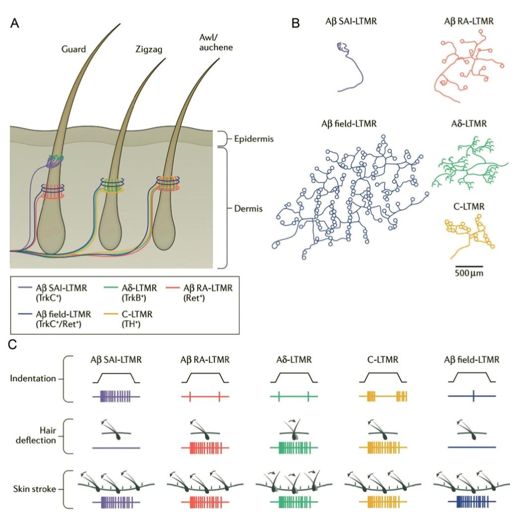
Figure 2.15 The mechanoreceptors of mammalian hairy skin. (A) Blanketing most of the body of mice and most mammals are several types of hairs (in mice, they are the guard, zigzag and awl/auchene hairs) that receive unique combinations of innervation by distinct low-threshold mechanoreceptor (LTMR) subsets. In mice, while the Ret-expressing (Ret+) Aẞ rapidly adapting (RA) LTMRS, TrkB-expressing (TrkB+) AS-LTMRs and TH-expressing (TH+) C-LTMRs all form lanceolate endings, the TrkC+/Ret+ Aẞ field-LTMRs form circumferential endings and the TrkC-expressing (TrkC+) Aẞ slowly adapting type 1 (SAI) LTMRs form touch domes with Merkel cells (shown in green). In mice (as shown here), the AB SAI-LTMRs form touch domes restricted to the mouth of the guard hair (the longest but least prevalent body hair); however, in humans, the AB SAI-LTMRs/touch domes are typically localized to skin between hair follicles. (B) A comparison of the peripheral terminals of individual, sparsely labelled LTMR subtypes in trunk hairy skin reveals that the lanceolate ending-forming and circumferential ending-forming LTMRs innervate numerous hair follicles (sometimes more than 100 hair follicles in the case of the Aẞ field-LTMR) over a large terminal area, unlike the AB SAI-LTMRs, which have a restricted terminal field area within the skin (usually associated with only a single guard hair in the mouse). The AS-LTMRs are unique in having polarized lanceolate endings around hair follicles that are restricted to the caudal (downward) side of zigzag and awl/auchene follicles. (C) Each LTMR subtype innervating hairy skin has a unique set of responses to common tactile stimuli. The responses shown here are schematic illustrations of typical responses. Although AB SAI-LTMRS, AB RA-LTMRS, A8-LTMRS, C-LTMRs and Aẞ field-LTMRs all respond to a stroke, which indents the skin and deflects multiple hairs as the stimulus moves across the surface of the skin, the AB SAI-LTMRs and Aẞ field-LTMRs are insensitive to deflection of individual hairs, and the AS-LTMRs are sensitive to deflection of awl/auchene or zigzag hairs in trunk skin specifically along the caudal-to-rostral axis and to deflection of the hairs in ventral paw skin along the rostral-to-caudal axis. The Aẞ field-LTMRs, while highly sensitive to gentle stroking across the skin, are relatively insensitive to skin indentation and thus exhibit indentation responses characteristic of high- threshold mechanoreceptors47. Although the AB SAI-LTMR, AB RA-LTMR, AS-LTMR and C-LTMRs all respond to skin indentation at low forces, their rates of adaptation vary, with the AB RA-LTMRS and AS-LTMRs adapting the fastest and the AB SAI-LTMRS the slowest. The Aẞ field- LTMRs adapt rapidly at the lowest indentation forces for which they do respond, while at high forces, the responses of the Aẞ field-LTMRs to indentation steps are more intermediately adapting and lack an off response ⁴⁷.
Credit: Fig. 2 of ref. 44. Part B was adapted by ref. 44 with permission from ref. 47.

شکل 2.15 گیرنده‌های مکانیکی پوست مودار پستانداران. (الف) بخش عمده‌ای از بدن موش‌ها و اکثر پستانداران را چندین نوع مو پوشانده است (در موش‌ها، این موها عبارتند از موهای محافظ، زیگزاگ و درفش/آوچن) که ترکیبات منحصر به فردی از عصب‌دهی را توسط زیرمجموعه‌های متمایز گیرنده‌های مکانیکی آستانه پایین (LTMR) دریافت می‌کنند. در موش‌ها، در حالی که LTMRSهای بیان‌کننده Ret (Ret+) Aẞ با سازگاری سریع (RA)، AS-LTMRهای بیان‌کننده TrkB (TrkB+) و C-LTMRهای بیان‌کننده TH (TH+) همگی انتهای نیزه‌ای تشکیل می‌دهند، LTMRهای میدانی TrkC+/Ret+ Aẞ انتهای محیطی تشکیل می‌دهند و LTMRهای نوع 1 بیان‌کننده TrkC (TrkC+) Aẞ با سازگاری آهسته (SAI) گنبدهای لمسی با سلول‌های مرکل (با رنگ سبز نشان داده شده‌اند) تشکیل می‌دهند. در موش‌ها (همانطور که در اینجا نشان داده شده است)، AB SAI-LTMRها گنبدهای لمسی را تشکیل می‌دهند که محدود به دهانه موی محافظ (طولانی‌ترین اما کم‌شایع‌ترین موی بدن) هستند. با این حال، در انسان، AB SAI-LTMRها/گنبدهای لمسی معمولاً در پوست بین فولیکول‌های مو قرار دارند. (ب) مقایسه پایانه‌های محیطی زیرگروه‌های LTMR منفرد و کم‌نشانه در پوست مودار تنه نشان می‌دهد که LTMRهای تشکیل‌دهنده انتهای نیزه‌ای و محیطی، فولیکول‌های موی متعددی (گاهی اوقات بیش از 100 فولیکول مو در مورد LTMR میدانی Aẞ) را در یک ناحیه ترمینال بزرگ عصب‌دهی می‌کنند، برخلاف AB SAI-LTMRها که دارای یک ناحیه میدان ترمینال محدود در پوست هستند (که معمولاً فقط با یک موی محافظ در موش مرتبط است). AS-LTMRها در داشتن پایانه‌های نیزه‌ای قطبی‌شده در اطراف فولیکول‌های مو که محدود به سمت دمی (رو به پایین) فولیکول‌های زیگزاگ و درفش/آوچن هستند، منحصر به فرد هستند. (ج) هر زیرگروه LTMR که پوست مودار را عصب‌دهی می‌کند، مجموعه‌ای منحصر به فرد از پاسخ‌ها را به محرک‌های لمسی رایج دارد. پاسخ‌های نشان داده شده در اینجا، تصاویر شماتیک از پاسخ‌های معمول هستند. اگرچه AB SAI-LTMRS، AB RA-LTMRS، A8-LTMRS، C-LTMRها و Aẞ field-LTMRها همگی به ضربه پاسخ می‌دهند که باعث فرورفتگی پوست و انحراف چندین مو هنگام حرکت محرک در سطح پوست می‌شود، AB SAI-LTMRها و Aẞ field-LTMRها به انحراف موهای منفرد حساس نیستند و AS-LTMRها به انحراف موهای درفش/آوچن یا زیگزاگ در پوست تنه به طور خاص در امتداد محور دمی به سری و به انحراف موها در پوست پنجه شکمی در امتداد محور سری به سری حساس هستند. گیرنده‌های LTMR میدان Aẞ، اگرچه به نوازش ملایم روی پوست بسیار حساس هستند، اما نسبت به فرورفتگی پوست نسبتاً غیرحساس هستند و بنابراین پاسخ‌های فرورفتگی مشخصه گیرنده‌های مکانیکی آستانه بالا را نشان می‌دهند47. اگرچه AB SAI-LTMR، AB RA-LTMR، AS-LTMR و C-LTMR همگی به فرورفتگی پوست در نیروهای کم پاسخ می‌دهند، سرعت سازگاری آنها متفاوت است، به طوری که AB RA-LTMRS و AS-LTMRها سریع‌ترین و AB SAI-LTMRها کندترین سازگاری را دارند. گیرنده‌های LTMR میدان Aẞ در کمترین نیروهای فرورفتگی که به آنها پاسخ می‌دهند، به سرعت سازگار می‌شوند، در حالی که در نیروهای بالا، پاسخ‌های گیرنده‌های LTMR میدان Aẞ به مراحل فرورفتگی، سازگاری متوسط‌تری دارند و فاقد پاسخ خاموش هستند ⁴⁷.
منبع: شکل 2 از مرجع 44. قسمت B توسط مرجع 44 با اجازه مرجع 47 اقتباس شده است.

2.6 Summary

From marine animals, insects to humans, we are all limited and shielded by the spatiotemporal resolution of our senses, which underlie what we remember and respond to. As long as an organism gets the necessary information for what it needs to do (e.g., bacterial chemotaxis⁴⁸), more information is not necessarily better. It is probably a universal theme that individual functions are achieved with a relatively small number of neurons. The sensory input sparsely and locally activates some of the neurons. Different inputs can be correlated and tracked. At the sensory end, the neural system is likely already a bottom-up setup that detects useful information (even when asleep, Chapter 6), while it can be modulated by a general status communicated as an integrated message.

۲.۶ خلاصه

از حیوانات دریایی، حشرات گرفته تا انسان‌ها، همه ما محدود و توسط تفکیک مکانی-زمانی حواس خود محافظت می‌شویم، که زیربنای آنچه را که به خاطر می‌آوریم و به آن پاسخ می‌دهیم، می‌باشد. تا زمانی که یک موجود زنده اطلاعات لازم را برای کاری که باید انجام دهد (مثلاً کموتاکسی باکتریایی۴۸) دریافت کند، اطلاعات بیشتر لزوماً بهتر نیست. احتمالاً یک موضوع جهانی است که عملکردهای فردی با تعداد نسبتاً کمی نورون حاصل می‌شوند. ورودی حسی به طور پراکنده و محلی برخی از نورون‌ها را فعال می‌کند. ورودی‌های مختلف را می‌توان همبسته و ردیابی کرد. در انتهای حسی، سیستم عصبی احتمالاً از قبل یک ساختار پایین به بالا است که اطلاعات مفید را تشخیص می‌دهد (حتی هنگام خواب، فصل ۶)، در حالی که می‌تواند توسط یک وضعیت کلی که به عنوان یک پیام یکپارچه منتقل می‌شود، تعدیل شود.

Questions

سوالات

1. How many steps do you think are needed from input to function for each sense?

۱. به نظر شما برای هر حس، از ورودی تا عملکرد، چند مرحله لازم است؟

2. When a group of cells become more sensitive to a particular input, what would be a good distribution of very sensitive cells and slightly more sensitive cells? How easily should they be reallocated to be more sensitive to another input?

۲. وقتی گروهی از سلول‌ها به یک ورودی خاص حساس‌تر می‌شوند، توزیع مناسب سلول‌های بسیار حساس و سلول‌های کمی حساس‌تر چگونه خواهد بود؟ چقدر آسان می‌توان آن‌ها را مجدداً تخصیص داد تا به ورودی دیگری حساس‌تر شوند؟

3. What other information from the environment could be useful for an animal, and how might that be sensed?

۳. چه اطلاعات دیگری از محیط می‌تواند برای یک حیوان مفید باشد و چگونه می‌توان آن را حس کرد؟

(Neuroscience for Artificial Intelligence
Huijue Ji

(علوم اعصاب برای هوش مصنوعی
هویجوئه جیا)

References

1. Fuscà, D. & Kloppenburg, P. Odor processing in the cockroach antennal lobe-the network components. Cell Tissue Res. 383, 59-73 (2021).
2. Shen, Y., Dasgupta, S. & Navlakha, S. Algorithmic insights on continual learning from fruit flies (2021). https://doi.org/10.48550/ arXiv.2107.07617.
3. Liang, Y. et al. Can a Fruit Fly Learn Word Embeddings? (2021). https://doi.org/10.48550/arXiv.2101.06887.
- Dasgupta, S., Stevens, C. F. & Navlakha, S. A neural algorithm for a fundamental computing problem. Science (80-.). 358, 793-796 (2017).
- DH, G., V, K., A, A.-A., A, S. & VN, M. Mice develop efficient strategies for foraging and navigation using complex natural stimuli. Curr. Biol. 26, 1261-1273 (2016).
- Bao, X. et al. Grid-like neural representations support olfactory navigation of a two-dimensional odor space. Neuron 102, 1066-1075. e5 (2019).
- Wu, Y., Chen, K., Ye, Y., Zhang, T. & Zhou, W. Humans navigate with stereo olfaction. Proc. Natl. Acad. Sci. 117, 16065-16071 (2020).
- Ackels, T. et al. Fast odour dynamics are encoded in the olfactory system and guide behaviour. Nature 593, 558-563 (2021).
- Pearl, J. & Mackenzie, D. The Book of Why (Basic Books, 2018).
- KC, C. Stereo and serial sniffing guide navigation to an odour source in a mammal. Nat. Commun. 4 (2013).
- Roper, S. D. & Chaudhari, N. Taste buds: cells, signals and synapses. Nat. Rev. Neurosci. 18, 485-497 (2017).
- Demi, L. M., Taylor, B. W., Reading, B. J., Tordoff, M. G. & Dunn, R. R. Understanding the evolution of nutritive taste in animals: insights from biological stoichiometry and nutritional geometry. Ecol. Evol. 11, 8441-8455 (2021).
- Yarmolinsky, D. A., Zuker, C. S. & Ryba, N. J. P. Common Sense about Taste: from Mammals to Insects. Cell 139, 234-244 (2009).
- Dotson, C. D., Shaw, H. L., Mitchell, B. D., Munger, S. D. & Steinle, N. I. Variation in the gene TAS2R38 is associated with the eating behavior disinhibition in Old Order Amish women. Appetite 54, 93-99 (2010).
- Ahn, J. E., Chen, Y. & Amrein, H. Molecular basis of fatty acid taste in Drosophila. Elife 6 (2017).
- Li, R. et al. The sequence and de novo assembly of the giant panda genome. Nature 463, 311-7 (2010).
- Feng, P. & Zhao, H. Bin. Complex evolutionary history of the vertebrate sweet/umami taste receptor genes. Chinese Sci. Bull. 58, 2198-2204 (2013).
- Kim, M., Heo, G. & Kim, S.-Y. Neural signalling of gut mechanosensation in ingestive and digestive processes. Nat. Rev. Neurosci. 23, 135-156 (2022).
- Jasmin, K., Lima, C. F. & Scott, S. K. Understanding rostral-caudal auditory cortex contributions to auditory perception. Nat. Rev. Neurosci. 20, 425-434 (2019).
- Moser, T., Grabner, C. P. & Schmitz, F. Sensory processing at ribbon synapses in the retina and the cochlea. Physiol. Rev. 100, 103-144 (2020).
- van der Heijden, K., Rauschecker, J. P., de Gelder, B. & Formisano, E. Cortical mechanisms of spatial hearing. Nat. Rev. Neurosci. 20, 609-623 (2019).
- Llorca, P. M. et al. Hallucinations in schizophrenia and Parkinson’s disease: an analysis of sensory modalities involved and the repercussion on patients. Sci. Rep. 6, 38152 (2016).
- Horga, G. & Abi-Dargham, A. An integrative framework for perceptual disturbances in psychosis. Nat. Rev. Neurosci. 20, 763-778 (2019).
- Silverstein, S. M. & Rosen, R. Schizophrenia and the eye. Schizophr. Res. Cogn. 2, 46-55 (2015).
- Marshel, J. H., Garrett, M. E., Nauhaus, I. & Callaway, E. M. Functional specialization of seven mouse visual cortical areas. Neuron 72, 1040-1054 (2011).
- Goltstein, P. M., Reinert, S., Bonhoeffer, T. & Hübener, M. Mouse visual cortex areas represent perceptual and semantic features of learned visual categories. Nat. Neurosci. 24, 1441-1451 (2021).
- Higgins, I. et al. Unsupervised deep learning identifies semantic disentanglement in single inferotemporal face patch neurons. Nat. Commun. 12, 6456 (2021).
- Bennett, C. et al. Higher-order thalamic circuits channel parallel streams of visual information in mice. Neuron 102, 477-492.e5 (2019).
- D’Souza, R. D. et al. Hierarchical and nonhierarchical features of the mouse visual cortical network. Nat. Commun. 13,503 (2022).
- G, D. et al. Perirhinal input to neocortical layer 1 controls learning. Science 370 (2020).
- Peng, H. et al. Morphological diversity of single neurons in molecularly defined cell types. Nature 598, 174-181 (2021).
- Karimi, A., Odenthal, J., Drawitsch, F., Boergens, K. M. & Helmstaedter, M. Cell-type specific innervation of cortical pyramidal cells at their apical dendrites. Elife 9 (2020).
- Roth, M. M. et al. Thalamic nuclei convey diverse contextual information to layer 1 of visual cortex. Nat. Neurosci. 19, 299-307 (2016).
- AW, I., Y, K. & Y, Y. Experience-Dependent Development of Feature-Selective Synchronization in the Primary Visual Cortex. J. Neurosci. 38, 7852-7869 (2018).
- Goll, Y., Atlan, G. & Citri, A. Attention: the claustrum. Trends Neurosci. 38, 486-95 (2015).
- Campagnola, L. et al. Local connectivity and synaptic dynamics in mouse and human neocortex. Science (80-.). 375 (2022).
- Arcaro, M. J. & Livingstone, M. S. On the relationship between maps and domains in inferotemporal cortex. Nat. Rev. Neurosci. 22, 573-583 (2021).
- Balcombe, J. What a Fish Knows: The Inner Lives of Our Underwater Cousins (Scientific American, 2017).
- Van der Velden, J., Zheng, Y., Patullo, B. W. & Macmillan, D. L. Crayfish recognize the faces of fight opponents. PLoS One 3, e1695 (2008).
- Norman, Y. et al. Hippocampal sharp-wave ripples linked to visual episodic recollection in humans. Science 365 (2019).
- Hesse, J. K. & Tsao, D. Y. The macaque face patch system: a turtle’s underbelly for the brain. Nat. Rev. Neurosci. 21, 695-716 (2020).
- Bao, P., She, L., McGill, M. & Tsao, D. Y. A map of object space in primate inferotemporal cortex. Nature 583, 103-108 (2020).
- Harris, C. M. et al. Gradients in mechanotransduction of force and body weight in insects. Arthropod Struct. Dev. 58, 100970 (2020).
- Handler, A. & Ginty, D. D. The mechanosensory neurons of touch and their mechanisms of activation. Nat. Rev. Neurosci. 22, 521-537 (2021).
- Lehnert, B. P. et al. Mechanoreceptor synapses in the brainstem shape the central representation of touch. Cell 184, 5608-5621.e18 (2021).
- Petersen, C. C. H. Sensorimotor processing in the rodent barrel cortex. Nat. Rev. Neurosci. 20, 533-546 (2019).
- Bai, L. et al. Genetic identification of an expansive mechanoreceptor sensitive to skin stroking. Cell 163, 1783-1795 (2015).
- Mattingly, H. H., Kamino, K., Machta, B. B. & Emonet, T. Escherichia coli chemotaxis is information limited. Nat. Phys. 17, 1426-1431 (2021).
📘 کتاب علوم اعصاب برای هوش مصنوعی
- نویسنده: Huijue Jia
- قالب فایل: PDF
- انتشارات: Jenny Stanford
- زبان اصلی: English
- سال انتشار: 2023